SGT for mixtures and \(\beta_{ij} \neq 0\)
When working with mixtures and at least one \(\beta_{ij} \neq 0\), SGT has to be solved as a boundary value problem (BVP)with a finite interfacial lenght.
In phasepy two solution procedure are available for this purpose, both on them relies on orthogonal collocation. The first one, solve the BVP at a given interfacial lenght, then it computes the interfacial tension. After this first iteration the interfacial lenght is increased and the density profiles are solved again using the obtained solution as an initial guess, then the interfacial tension is computed again. This iterative procedure is repeated until the interfacial tension stops decreasing whithin a given tolerance (default value 0.01 mN/m). This procedure is inspired in the work of Liang and Michelsen.
First, as for any SGT computation, equilibria has to be computed.
>>> hexane = component(name = 'n-Hexane', Tc = 507.6, Pc = 30.25, Zc = 0.266, Vc = 371.0, w = 0.301261,
                ksv = [ 0.81185833, -0.08790848],
                cii = [ 5.03377433e-24, -3.41297789e-21,  9.97008208e-19],
                GC = {'CH3':2, 'CH2':4})
>>> ethanol = component(name = 'Ethanol', Tc = 514.0, Pc = 61.37, Zc = 0.241, Vc = 168.0, w = 0.643558,
                ksv = [1.27092923, 0.0440421 ],
                cii = [ 2.35206942e-24, -1.32498074e-21,  2.31193555e-19],
                GC = {'CH3':1, 'CH2':1, 'OH(P)':1})
>>> mix = mixture(ethanol, hexane)
>>> a12, a21 = np.array([1141.56994427,  125.25729314])
>>> A = np.array([[0, a12], [a21, 0]])
>>> mix.wilson(A)
>>> eos = prsveos(mix, 'mhv_wilson')
>>> T = 320 #K
>>> X = np.array([0.3, 0.7])
>>> P0 = 0.3 #bar
>>> Y0 = np.array([0.7, 0.3])
>>> sol = bubblePy(Y0, P0, X, T, eos, full_output = True)
>>> Y = sol.Y
>>> P = sol.P
>>> vl = sol.v1
>>> vv = sol.v2
>>> #computing the density vector
>>> rhol = X / vl
>>> rhov = Y / vv
The correction \(\beta_{ij}\) has to be supplied to the eos with eos.beta_sgt method. Otherwise the influence parameter matrix will be singular and a error will be raised.
>>> bij = 0.1
>>> beta = np.array([[0, bij], [bij, 0]])
>>> eos.beta_sgt(beta)
Then the interfacial tension can be computed as follows:
>>> sgt_mix(rhol, rhov, T, P, eos, z0 = 10.,  rho0 = 'hyperbolic', full_output = False)
>>> #interfacial tension in mN/m
>>> 14.367813285945807
In the example z0 refers to the initial interfacial langht, rho0 refers to the initial guess to solve the BVP. Available options are 'linear' for linear density profiles, hyperbolic for density profiles obtained from hyperbolic tangent. Other option is to provide an array with the initial guess, the shape of this array has to be nc x n, where n is the number of collocation points. Finally, a TensionResult can be passed to rho0, this object is usually obtained from another SGT computation, as for example from a calculation with \(\beta_{ij} = 0\).
If the full_output option is set to True, all the computated information will be given in a TensionResult object. Atributes are accessed similar as SciPy OptimizationResult.
>>> sol = sgt_mix(rhol, rhov, T, P, eos, z0 = 10.,  rho0 = 'hyperbolic', full_output = False)
>>> sol.tension
... 14.36781328594585 #IFT in mN/m
>>> #density profiles and spatial coordiante access
>>> sol.rho
>>> sol.z
-
sgt_mix(rho1, rho2, Tsat, Psat, model, rho0='linear', z0=10.0, dz=1.5, itmax=10, n=20, full_output=False, ten_tol=0.01, root_method='lm', solver_opt=None)[source]¶ SGT for mixtures and beta != 0 (rho1, rho2, T, P) -> interfacial tension
Parameters: - rho1 (float) – phase 1 density vector
- rho2 (float) – phase 2 density vector
- Tsat (float) – saturation temperature
- Psat (float) – saturation pressure
- model (object) – created with an EoS
- rho0 (string, array_like or TensionResult) – inital values to solve the BVP, avaialable options are ‘linear’ for linear density profiles, ‘hyperbolic’ for hyperbolic like density profiles. An array can also be supplied or a TensionResult of a previous calculation.
- z0 (float) – initial interfacial lenght
- dz (float) – increase in interfacial lenght per interation
- itmax (int) – maximun number of iterations
- n (int, optional) – number points to solve density profiles
- full_output (bool, optional) – wheter to outputs all calculation info
- root_method (string, optional) – Method used un SciPy’s root function default ‘lm’, other options: ‘krylov’, ‘hybr’. See SciPy documentation for more info
- solver_opt (dict, optional) – aditional solver options passed to SciPy solver
Returns: ten – interfacial tension between the phases
Return type: float
The second solution method is based on a modified SGT system of equations, proposed by Mu et al. This system introduced a time variable \(s\) which helps to get linearize the system of equations during the first iterations.
This differential equation is advanced in time until no further changes is found on the density profiles. Then the interfacial tension is computed.
Its use is similar as the method described above, with the msgt_mix function.
>>> solm = msgt_mix(rhol, rhov, T, P, eos, z = 20, rho0 = sol, full_output = True)
>>> solm.tension
... 14.367827924919165 #IFT in mN/m
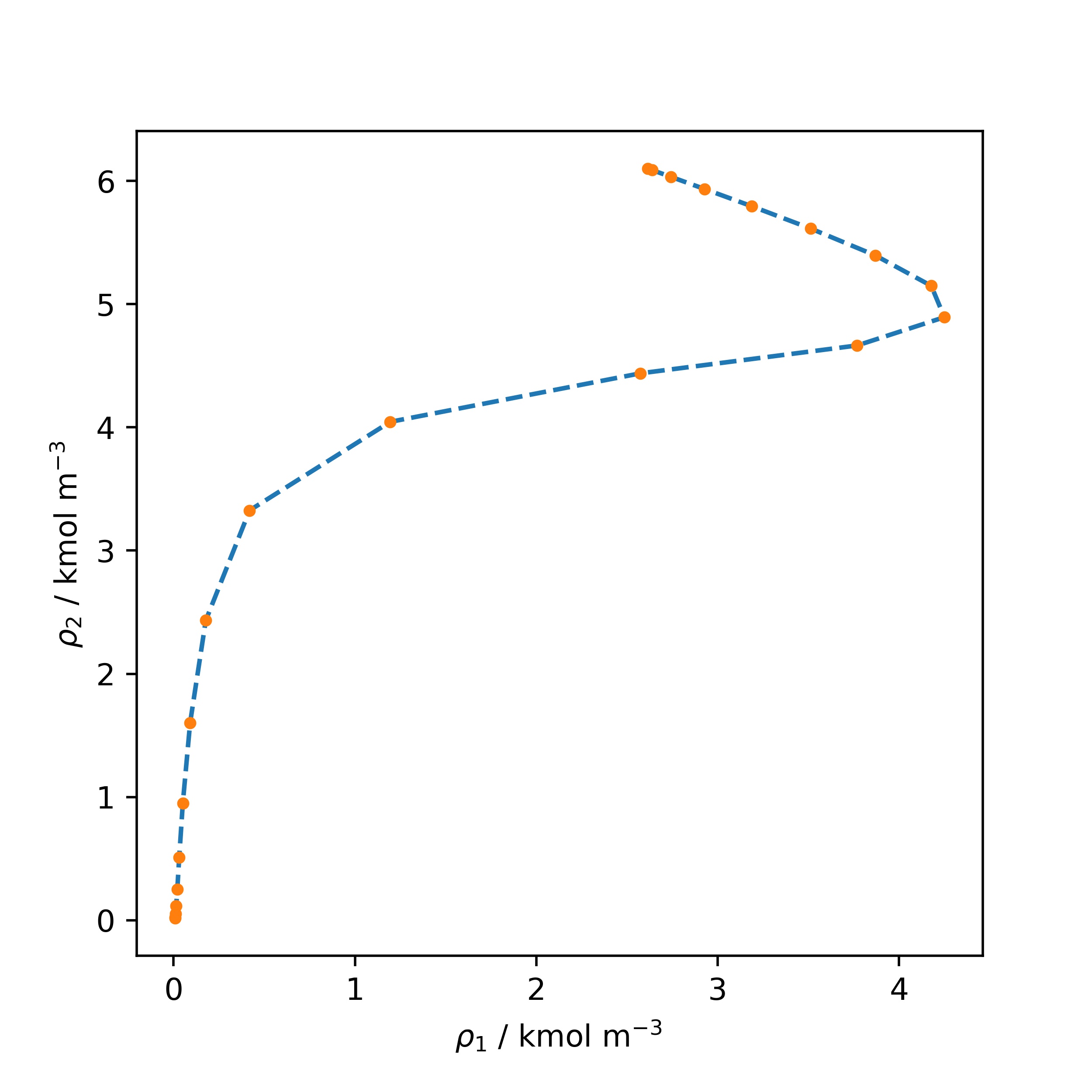
The density profiles obtained from each method are show in the following figure. The dashed line was computed solving the original BVP with increasing interfacial length and the dots were computed with the modified system.
-
msgt_mix(rho1, rho2, Tsat, Psat, model, rho0='linear', z=20.0, n=20, ds=0.1, itmax=30, rho_tol=0.01, full_output=False, root_method='lm', solver_opt=None)[source]¶ SGT for mixtures and beta != 0 (rho1, rho2, T, P) -> interfacial tension
Parameters: - rho1 (float) – phase 1 density vector
- rho2 (float) – phase 2 density vector
- Tsat (float) – saturation temperature
- Psat (float) – saturation pressure
- model (object) – created with an EoS
- rho0 (string, array_like or TensionResult) – inital values to solve the BVP, avaialable options are ‘linear’ for linear density profiles, ‘hyperbolic’ for hyperbolic like density profiles. An array can also be supplied or a TensionResult of a previous calculation.
- z (float, optional) – initial interfacial lenght
- n (int, optional) – number points to solve density profiles
- ds (float, optional) – time variable integration delta
- itmax (int, optional) – maximun number of iterations foward on time
- rho_tol (float, optional) – desired tolerance for density profiles
- full_output (bool, optional) – wheter to outputs all calculation info
- root_method (string, optional) – Method used un SciPy’s root function default ‘lm’, other options: ‘krylov’, ‘hybr’. See SciPy documentation for more info
- solver_opt (dict, optional) – aditional solver options passed to SciPy solver
Returns: ten – interfacial tension between the phases
Return type: float